Quaternions are a nifty way to represent rotations in 3D space. You can find many introductions to quaternions out there on the internet, so I'm going to assume you know the basics. For a refresher, see the papers by Shoemake or Eberly in the References.In this article we will look closely at the tasks of quaternion interpolation and normalization, and we'll develop some good tricks.
When game programmers want to interpolate between quaternions, they tend to copy Ken Shoemake's code without really understanding it. Ken uses a function called slerp that walks along the unit sphere in 4-dimensional space from one quaternion to the other. Because it's navigating a sphere, it involves a fair amount of trigonometry, and is correspondingly slow.Lacking a strong grasp of quaternions, most game developers just accept this: slerp is slow, and if you want something faster, maybe you should go back to Euler angles and all their nastiness. But the situation is not so bad. There's a cheap approximation to slerp that will work in most cases, and is so braindead simple and fast that it's shocking. Shocking, I tell you.
Slerp is desirable because of two main properties; any approximation we formulate would ideally have the same properties. The first, and perhaps most important, is that slerp produces the shortest path between the two orientations on that unit sphere in 4D; this is equivalent to finding the "minimum torque" rotation in 3D space, which you can think of as the smoothest transition between two orientations. The second property of slerp is that it travels this path at a constant speed, which basically means you have full control over the nature of the transition (if you want to add some style, like starting slowly and then speeding up, you can just spline your time parameter before feeding it into slerp.)
So here's our approximation: linearly interpolate the two quaternions, componentwise. That is, if t is your time parameter from 0 to 1, then $x=x_0+t(x_1-x_0)$, and similarly for y, z, and w.
One might say: Ridiculous! How could that possibly be a worthwhile interpolation, when the "right answer" is so much more complicated? Let's take a look.
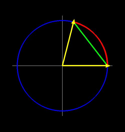
Figure 1 shows a 2-dimensional version of quaternion interpolation. Slerp walks around the edge of the unit circle, which is what we want. Linear interpolation results in a chord that cuts inside the circle. But here's the thing to realize: normalizing all the points along the chord stretches them out to unit length, so that they lie along the slerp path. To restate: if you linearly interpolate two quaternions from t = 0 to t = 1, and then normalize the result, you get the same minimal-torque transition that slerp would have given you.

Figure 1: A 2-dimensional picture of quaternion interpolation. The blue circle is the unit sphere; the two yellow vectors are the quaternions. The red arc represents the path traveled by slerp; the green chord shows the path taken by linear interpolation.
The Linear Algebra way to see this is that both the great circle and the chord lie in $\mathrm{{Span}(q_0,\ q_1)}$, which is a 2D subspace of the 4D embedding space. Adding the constraint that $\mathrm{Length(Interpolate(q_0,\ q_1,\ t)) = 1}$ reduces the dimensionality to one, so both paths must lie along the same circle. And both forms of interpolation produce only a continuous path of points between $\mathrm{q_0}$ and $\mathrm{q_1}$, so they must be the same. If $\mathrm{q_0}$ and $\mathrm{q_1}$ lie on opposing points of the sphere, the chord will pass through the origin and normalization will be undefined. But that's okay -- unless you're doing something wacky, you don't want your quaternions to be further than 90 degrees apart in the first place. (Because every rotation has 2 quaternion representations on the unit sphere, and you want to pick the closest ones to interpolate between.) So the normalization will always be well-defined. So the normalized linear interpolation and the slerp both trace out the same path. There is a difference between them, though: they travel at differing speeds. The linear interpolation will move quickly at the endpoints and slowly in the middle. Figure 2 shows a graph of the worst case, 90 degrees.The function graphed in Figure 2 is
$$ \tan^{-1}{t\sin{a}\over{1+t(\cos{a}-1)}} $$
where α is the original angle between the two quaternions. I figured this out just by drawing a 2D graph like Figure 1, where one of my vectors is the x axis (1, 0) and the other one is $(\cos{a},\ \sin{a})$. Then I just wrote an expression for linearly interpolating between them by 't', and then finding the resulting angle by $\tan^{-1}$. This rather simplistic approach is valid because: (a) since all the action happens in $\mathrm{Span(q_0,\ q_1)}$, we can just take that 2D cross-section out of 4D space; studying it in isolation, we see the entirety of what is happening. And (b) on the resulting 2D unit circle, because the set of all possibilities for the two unit vectors is redundant by rotational symmetry, we can choose one of the vectors to be anything we like; I chose (1, 0) to simplify the math.
Casey Muratori is the first person I know of who considered linear interpolation of quaternions as a serious option. He investigated numerically and found linear interpolation, when properly employed, to be quite worthwhile. So hats off to Casey, eh? Casey makes the animation toolkit Granny 2 (by RAD Game Tools), and he has eradicated all slerps from his code. Granny 2 never slerps at runtime, which is pretty cool considering all the stuff it does.

Figure 2: Worst case of lerp speed variation. Green: ideal result produced by slerp; Red: distorted result produced by lerp. The error between these two functions should be measured vertically, so they are more different than they may appear at first.

Figure 3: The compensating cubic spline, k = 0.45, shown in yellow atop the graph of figure 2.
The linear interpolation is monotonic from $\mathrm{q_1}$ to $\mathrm{q_2}$, so if you are doing an application where you're binary searching for a result that satisfies some constraint, using the linear interpolation works just fine. If your quaternions are very close together (under 30 degrees, say), as you have when playing back a series of time-sampled animation data, linear interpolation works fine. And if you have some number of different character poses (like an enemy pointing his gun in several different directions), and you want to mix them based on a blending parameter, linear interpolation probably works fine.
Linear interpolation won't work if you need precise speed control and wide interpolation angles. But maybe we can fix that.
Perhaps we can make a spline that cancels most of the speed distortion. Looking at Figure 2, can we concoct a function that, when multiplied against the curve, causes it to lie much closer to the ideal line? The way I chose to visualize this was with a cubic spline that tries to pull the distortion function onto the diagonal. Figure 3 shows a cubic spline with the equation $y=2kt^3-3kt^2+(1+k)t$, where the tuning parameter k = 0.45, graphed against the plot of figure 2. [Note: We are looking for some function g to help us correct f; strictly speaking, the most general approach is to structure the correction as g(f(t)), not g(t)f(t). But I can get away with thinking of this correction as a multiplication problem because: (1) In this case f(t) = t, and (2) I'm using splines with no constant coefficients, so I can factor t out of the spline. Essentially I used some foreknowledge about the nature of the solution to simplify the problem.]
Because both the distortion curve and our compensating spline have an average value of 't', and are approximately complementary, when we multiply them together we get a function that is approximately $g(t)=t^2$. We want $g(t)=t$, so we'll divide the cubic spline by t. Fortunately, since the spline passes through the origin, it has no 'd' coefficient; so dividing by t just turns it into a quadratic curve: $y=2kt^2-3kt+1+k$.
So now, if we're linearly interpolating two splines that are 90 degrees apart, we find $t'=2kt^2-3kt+1+k$, and use t' as our interpolation parameter. We get something very close to constant-speed interpolation (I will quantify how close in a little bit). However, if we reduce the angle between the input quaternions, we get something that's less accurate than the original 't'.